Cross-validation for restricted bridge regression

Evaluate a fitted penalty path using contiguous validation folds and return the full-data coefficients together with two penalty selectors.

Usage

cv.rbridge(
  X,
  y,
  q,
  R,
  r,
  lambda,
  nfolds = 10,
  lambda.min = ifelse(n > p, 0.001, 0.05),
  nlambda = 100,
  eta = 1e-07,
  converge = 10^10,
  num_threads = 10
)

Arguments

X: Numeric design matrix with n observation rows and p predictor columns. Supply finite values and predictors with nonzero variation; omit an intercept column. A data frame is converted using model.matrix(~0+., X); restrictions and future predictions must use the resulting predictor order.
y: Numeric response vector of length n, containing finite values.
q: Bridge-penalty exponent, a finite number in (0, 2]. Values 1 and 2 specify the L1 and L2 penalty forms. Estimation uses local quadratic approximation (LQA).
R: Finite numeric matrix with m linearly independent restriction rows and p predictor columns. Each row specifies a linear combination of the standardized predictor coefficients, in the order of X. The intercept is excluded.
r: Finite numeric target vector of length m, or an m by 1 matrix. The targets have the units of the response when R is dimensionless. See Details for the coefficient scale and a residual check.
lambda: Optional nonempty numeric vector of finite, nonnegative penalty values. Its order is retained. When supplied, it determines the fitted path and overrides nlambda and the grid argument lambda.min.
nfolds: Number of validation folds, an integer between 2 and n. The default is 10.
lambda.min: Positive absolute endpoint of the automatically generated penalty grid. The default is 0.001 when n > p, and 0.05 otherwise. This argument is a penalty value, not a ratio. In CV results, the field also named lambda.min instead denotes the selected penalty.
nlambda: Number of automatically generated penalty values, an integer of at least 2. The default is 100; ignored when lambda is supplied.
eta: Positive numerical tolerance, with default 1e-7. Used for coefficient elimination and stopping on squared coefficient changes.
converge: Nonnegative initial convergence-distance value, retained for compatibility. The default is 1e10. Iteration stops when the updated squared coefficient change is at most eta, or at the historical cap.
num_threads: Requested fold-level workers, a positive integer. The default is 10; the effective count is capped at nfolds. Builds without OpenMP execute folds sequentially. Use rbridge_info() to inspect the compiled support.

Value

A list of class cv.rbridge with components:

cve: Numeric vector of validation mean squared errors, one per penalty. Squared holdout residuals are summed across folds and divided by the total observation count, so each observation has the same weight.
cvse: Numeric vector from the historical CV error-bar calculation. It is not the conventional standard error of foldwise mean squared errors.
cvup, cvlo: Upper and lower curves, computed as cve + cvse and cve - cvse.
lambda: Numeric penalty vector in fitted order.
nz: Number of nonzero slopes, excluding the intercept, in each full-data fit.
betas: Full-data coefficient matrix with p + 1 rows and length(lambda) columns. The first row is (Intercept); the remaining rows are original-scale slopes in predictor order.
lambda.min: Fitted penalty with the smallest cve. Ties select the largest penalty among the minimizers. This selected value is distinct from the input argument specifying the generated grid endpoint.
lambda.1se: Largest fitted penalty whose cve is no greater than cve + cvse evaluated at the selected lambda.min. The name follows the historical convention; the threshold uses the package's cvse calculation described above.

Details

Fold assignment follows the supplied row order. The nfolds validation sets are contiguous blocks; their sizes can differ by one. Centering and RMS scaling use all observations before fold allocation, and each fold fit also reconstructs its training-set intercept. These historical preprocessing and error-bar conventions are retained. The reported validation error aggregates held-out predictions at each fitted penalty, and coefficients in betas come from a final fit to all observations.

For one fixed penalty, let $K$ be nfolds, $n$ the total observation count, $I_k$ the validation indices in fold $k$ , and $e_i$ the held-out response residual for observation $i$ . Equation (1) defines a fold's error contribution $d_k$ , the pooled validation MSE, and the historical error-bar width: $\begin{aligned} d_k&=\frac{1}{n}\sum_{i\in I_k}e_i^2,\\ \mathrm{cve}&=\sum_{k=1}^{K}d_k,\\ \mathrm{cvse}&=\sqrt{\frac{1}{K(n-1)} \sum_{k=1}^{K}(d_k-\mathrm{cve})^2}. \qquad (1) \end{aligned}$ The folds partition all observations, so the sum in Equation (1) weights each held-out observation equally. The final quantity supplies the plotted bar width and the historical lambda.1se threshold. Its centering uses the pooled cve, not the average fold contribution, and it is not a conventional foldwise standard error.

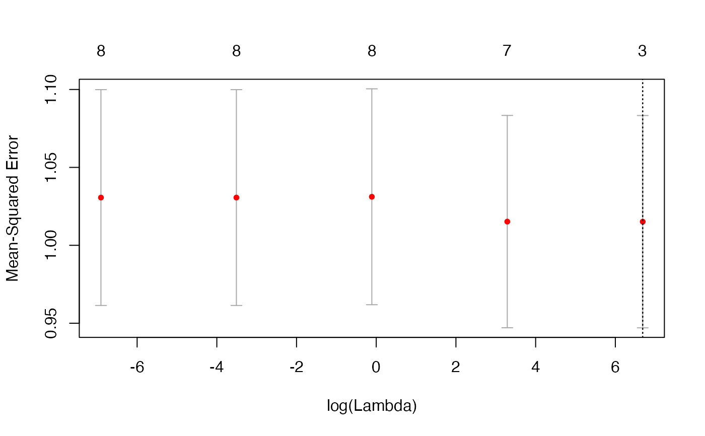
predict() defaults to the minimum-error penalty lambda.min. coef() defaults to lambda.1se. Supply s explicitly to use the same penalty for both operations. Use plot() to inspect the curve, error bars and selected penalties.

Restrictions act on standardized slopes. To check a fitted original-scale slope vector, multiply it elementwise by the centered RMS deviations of the predictors before applying R. The resulting restriction residual is the fitted linear combination minus r; it should be examined with a numerical tolerance, particularly after coefficient thresholding. For example, a zero restriction on one slope has the same meaning on either scale, whereas a nonzero sum or contrast depends on the scales.

Author

Bahadir Yuzbasi
Maintainer: Bahadir Yuzbasi b.yzb@hotmail.com

Examples

# Reproducible synthetic demonstration: 100 observations, eight predictors.
set.seed(2019)
beta <- c(3, 1.5, 0, 0, 2, 0, 0, 0)
p <- length(beta)
beta <- matrix(beta, nrow = p, ncol = 1)
n <- 100
X <- matrix(rnorm(n * p), nrow = n, ncol = p)
y <- as.numeric(X %*% beta + rnorm(n))
# A user-specified sum of standardized slopes: b[1] + b[2] + b[5] = 6.5.
# This target is illustrative; it is not asserted to equal the generating sum.
R1.mat <- matrix(c(1, 1, 0, 0, 1, 0, 0, 0), nrow = 1)
r1.vec <- matrix(6.5, nrow = 1, ncol = 1)
# A second standardized-slope contrast: -b[1] + b[2] + b[5] = 0.5.
R2.mat <- matrix(c(-1, 1, 0, 0, 1, 0, 0, 0), nrow = 1)
r2.vec <- matrix(0.5, nrow = 1, ncol = 1)
# Impose both independent restrictions together.
R3.mat <- rbind(R1.mat, R2.mat)
r3.vec <- matrix(c(6.5, 0.5), ncol = 1)
# Alternatively, set the five inactive generating slopes to zero.
p.active <- which(beta != 0)
R4.mat <- diag(p)[-p.active, , drop = FALSE]
r4.vec <- matrix(rep(0, p - length(p.active)), ncol = 1)

# Five penalties keep this help example fast; the default is 100.
# Three contiguous folds and one worker keep this demonstration small.
model1 <- cv.rbridge(X, y, q = 1, R = R1.mat, r = r1.vec,
                     nlambda = 5, nfolds = 3, num_threads = 1)
model2 <- cv.rbridge(X, y, q = 1, R = R2.mat, r = r2.vec,
                     nlambda = 5, nfolds = 3, num_threads = 1)
model3 <- cv.rbridge(X, y, q = 1, R = R3.mat, r = r3.vec,
                     nlambda = 5, nfolds = 3, num_threads = 1)
model4 <- cv.rbridge(X, y, q = 1, R = R4.mat, r = r4.vec,
                     nlambda = 5, nfolds = 3, num_threads = 1)
# Inspect both selectors and explicitly choose the minimum-error fit.
c(minimum_error = model1$lambda.min, historical_1se = model1$lambda.1se)
#>  minimum_error historical_1se 
#>       802.1497       802.1497 
coef(model1, s = "lambda.min")
#>             802.149726533951
#> (Intercept)       0.01283347
#> V1                2.98320054
#> V2                1.57870923
#> V3                0.00000000
#> V4                0.00000000
#> V5                1.99412306
#> V6                0.00000000
#> V7                0.00000000
#> V8                0.00000000
predict(model1, newx = X[1:5, , drop = FALSE], s = "lambda.min")
#> [1]  -1.6233986   0.3470059  -1.5648146   2.6330664 -10.4462475
plot(model1)

# Check the restriction after converting the returned slopes.
x_centered <- sweep(X, 2, colMeans(X), "-")
x_rms <- sqrt(colMeans(x_centered^2))
standardized_slopes <- coef(model1, s = "lambda.min")[-1, 1] * x_rms
as.numeric(R1.mat %*% standardized_slopes - r1.vec)
#> [1] 0