LHWR: Kernels, Bandwidth Selection and Diagnostics

What this guide covers

This companion to the introduction explains the decisions between supplying coordinates and reporting a fitted Gaussian LHWR model. The graphics gallery shows how to display the resulting quantities. The separate Lasso guide covers penalized tuning: its active sets and selection criteria must not be confused with unpenalized coefficient inference.

All examples are small, offline documentation checks, not a new empirical study. They reuse the introduction’s 141-country WDI 2024 sample, response, standardized regressors, stored representation and five-candidate grid. No observations are removed or imputed. Standardization below applies to the two regression predictors, not to the supplied Lorentz coordinates.

data("wdi_lhwr")
wdi <- subset(wdi_lhwr, year == 2024)
Z <- as.matrix(wdi[, c("z0_lorentz", "z1_lorentz", "z2_lorentz")])
dat <- data.frame(gdp_growth = wdi$gdp_growth,
  unemployment = as.numeric(scale(wdi$unemployment)),
  internet_users = as.numeric(scale(wdi$internet_users)))
form <- gdp_growth ~ unemployment + internet_users
candidate_k <- seq(30, 70, by = 10)
stopifnot(nrow(dat) == 141L, !anyNA(dat), nrow(Z) == nrow(dat))

Kernel shape is different from bandwidth

Let d_{ij}\geq0 be the chosen distance between observations i and j, and h_i>0 a local distance radius. Kernel weights are w_{ij}=K(u_{ij}), where u_{ij}=d_{ij}/h_i is dimensionless. The kernel sets how quickly influence decays with relative distance; the radius sets the scale of the neighbourhood. The five implemented functions are shown below for u\geq0. Compact kernels are zero at u=1, not only outside the radius.

Implemented kernel formulas for nonnegative relative distance.
Kernel	K(u)	Support
bisquare	(1-u²⁾2 for u<1; 0 otherwise	Compact
tricube	(1-u³⁾3 for u<1; 0 otherwise	Compact
boxcar	1 for u<1; 0 otherwise	Compact
gaussian	exp(-u^2/2)	Noncompact
exponential	exp(-u)	Noncompact

kernel_names <- c("bisquare", "tricube", "boxcar", "gaussian", "exponential")
u <- seq(0, 3, length.out = 301)
kernel_weights <- sapply(kernel_names, function(k) hgwr_kernel(u, 1, k))
kernel_cols <- c("#176B72", "#7B3294", "#D55E00", "#0072B2", "#6B6B00")
matplot(u, kernel_weights, type = "l", lty = seq_along(kernel_names),
        col = kernel_cols, lwd = 2, xlab = "Relative distance d / h",
        ylab = "Kernel weight", ylim = c(0, 1.05))
abline(v = 1, lty = 3, col = "grey65")
legend("topright", kernel_names, col = kernel_cols,
       lty = seq_along(kernel_names), lwd = 2, bty = "n", cex = 0.85)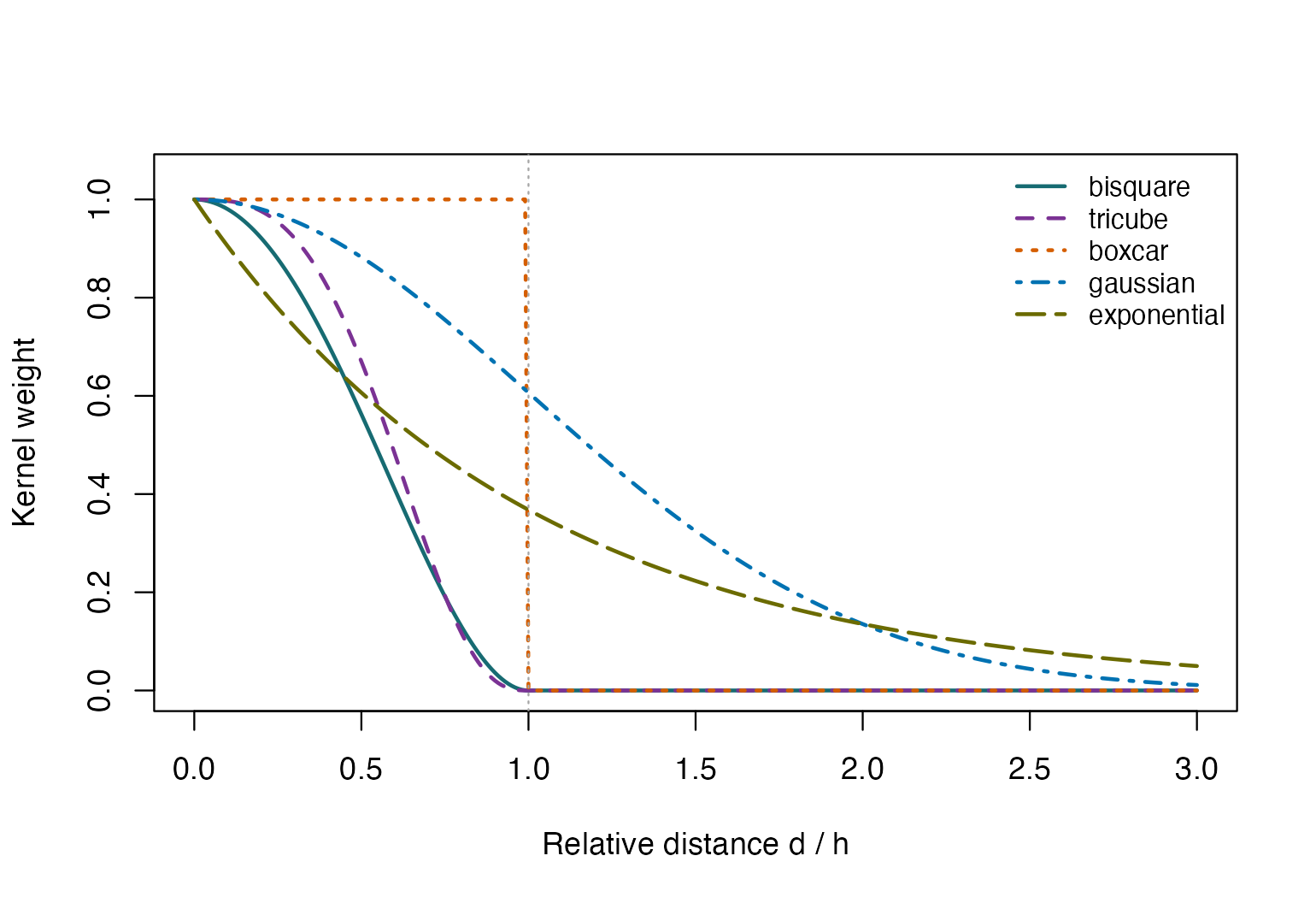

Kernel weights versus distance divided by bandwidth. Gaussian and exponential weights remain positive beyond the radius; the three compact kernels have zero boundary weight.

Changing a kernel changes the estimator. Comparing kernels requires the same analysis sample, representation and a declared selection protocol; these curves do not establish that one kernel is best. Do not truncate a Gaussian or exponential kernel merely to obtain a faster computation.

What `bw`, `adaptive` and `engine` mean

Bandwidth contracts. Volume options require Lorentz geometry.
Setting	Meaning of scalar bw	Engine
adaptive=TRUE, bandwidth_type=‘knn’	Target positive-distance neighbour rank k	dense or supported knn
adaptive=FALSE, bandwidth_type=‘knn’	Fixed distance radius h	dense
adaptive=FALSE, bandwidth_type=‘volume’	Fixed hyperbolic ball area V	dense
adaptive=TRUE, bandwidth_type=‘volume’	Target local mass; radius obtained using a pilot density	dense

For adaptive kNN bandwidths, the radius is the distance to the requested positive-distance neighbour rank. The focal observation has zero distance and is used in calibration, but does not count toward that positive-distance rank. Coincident points and boundary ties make bw different from the count of strictly positive regression weights. Inspect local_n_positive and local_neff rather than reporting bw as an effective sample size.

For the two-dimensional unit-curvature model, ball area and its inverse are V(h)=2\pi(\cosh h-1) and h(V)=\operatorname{arcosh}\{1+V/(2\pi)\}, for h,V\geq0. These convert between intrinsic radius and area. In adaptive-volume mode, pilot_k supplies the pilot neighbour rank used to estimate local point density; target mass divided by that density gives a target area, which is then inverted. This is a different bandwidth rule, not another name for kNN.

The kNN engine is a computational choice: exact Lorentz neighbours with adaptive kNN bandwidths and bisquare, tricube or boxcar kernels. It does not support tangent geometry, supplied dMat, fixed radii, volume bandwidths, Gaussian or exponential kernels. Use engine="dense" for those cases. The dense engine stores an n-by-n distance matrix; kNN reduces that storage, but some post-fit diagnostics still reconstruct dense operators. n_threads=1 is the reproducible serial default, not a statistical parameter.

AICc and CV select a bandwidth; AIC and BIC summarize a fit

For a Gaussian LHWR fit, let n be the sample size, S its conditional smoother matrix such that \widehat y=Sy, and R=\sum_i(y_i-\widehat y_i)^2>0 its residual sum of squares. Define t=\operatorname{tr}(S), the smoother trace. The implementation uses the Gaussian deviance-like quantity D=n\log(R/n)+n\log(2\pi)+n and the following information criteria:

\begin{aligned} \mathrm{AIC}&=D+2(t+1),\\ \mathrm{AICc}&=D+\frac{2n(t+1)}{n-t-2},\\ \mathrm{BIC}&=D+\log(n)(t+1). \end{aligned}\tag{1}

Equation (1) balances calibration fit and conditional model complexity; the extra one accounts for the variance parameter. AICc requires n-t-2>0; the package assigns an infinite score otherwise. The trace is not the number of predictors. These working smoother criteria do not add a penalty for learning the representation or searching over representations. Scores are comparable only under a common response, sample and likelihood convention; a smaller score is not a hypothesis-test p-value.

Gaussian CV instead evaluates \mathrm{CV}(b)=\sum_i\{y_i-\widehat y_{i,b}^{(-i)}\}^2, where b is a candidate bandwidth and \widehat y_{i,b}^{(-i)} omits observation i’s response from its local calibration. This is a sum of squared errors. The supplied coordinates and candidate neighbourhood radii remain fixed during this internal score. It is not an outer validation of an embedding-plus-tuning pipeline and does not reselect bandwidth inside each held-out case. Binary-response CV uses Bernoulli log loss instead; Gaussian AICc and F diagnostics are not defined for binomial fits.

bw_aicc <- bw.lhwr(form, dat, Z = Z, bw_grid = candidate_k,
                   approach = "AICc", kernel = "bisquare", engine = "knn")
bw_cv <- bw.lhwr(form, dat, Z = Z, bw_grid = candidate_k,
                 approach = "CV", kernel = "bisquare", engine = "knn")
knitr::kable(data.frame(Criterion = c("AICc", "CV"),
  Selected_k = c(bw_aicc$bw, bw_cv$bw),
  Score = c(bw_aicc$score, bw_cv$score)), digits = 3,
  caption = "Two criteria applied to exactly the same five candidates.")

Two criteria applied to exactly the same five candidates.
Criterion	Selected_k	Score
AICc	40	622.824
CV	30	685.267

plot_lhwr_diagnostics(bw_aicc, type = "bandwidth")
plot_lhwr_diagnostics(bw_cv, type = "bandwidth")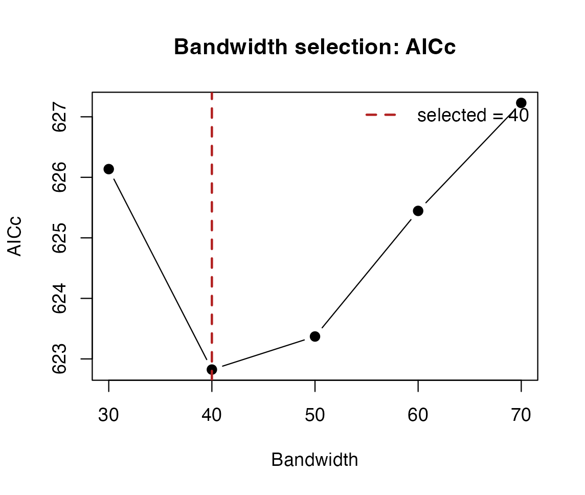

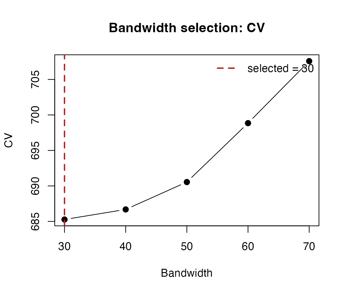
Left: AICc. Right: leave-one-out squared-error CV over the same neighbour counts. Vertical scales differ because the criteria have different units.

bw.lhwr() accepts approach="AICc" or "CV", not "AIC" or "BIC". AIC and BIC can be extracted after fitting. An explicit bw_grid selects grid search; otherwise the default is golden-section search over an interval controlled by lower, upper, tol and max_iter. The selected minimum is among evaluated candidates, not proof of a global minimum over every possible bandwidth. Boundary selections warrant review of support and search range, not automatic widening until a desired result appears. selection.table records the evaluated candidates and scores.

fit <- lhwr(form, dat, Z = Z, bw = bw_aicc$bw, kernel = "bisquare",
            engine = "knn", diagnostics = "full", f_tests = FALSE)
diag_fit <- fit$LHWR.diagnostic
knitr::kable(data.frame(Quantity = c("RSS", "AIC", "AICc", "BIC", "tr(S)", "edf"),
  Value = unlist(diag_fit[c("RSS.gw", "AIC", "AICc", "BIC", "tr.S", "edf")])),
  digits = 3, caption = "Post-fit Gaussian diagnostics from the AICc-selected fit.")

Post-fit Gaussian diagnostics from the AICc-selected fit.
	Quantity	Value
RSS.gw	RSS	456.092
AIC	AIC	612.854
AICc	AICc	622.824
BIC	BIC	682.428
tr.S	tr(S)	22.594
edf	edf	110.958

CV.lhwr(bw_cv)
#> [1] 685.2671

CV.lhwr(fit) may return NA when no CV score was computed for that object; it does not start a new cross-validation. Likewise diagnostics="none" does not contain the hat-matrix quantities needed for AICc or F tests. diagnostics="aicc" computes trace-based summaries but omits local standard errors; "full" supplies the local inference quantities used below.

Local design and coefficient uncertainty

For weights w_{ij}, effective local support is n_{\mathrm{eff},i}=(\sum_j w_{ij})^2/\sum_j w_{ij}^2, provided the denominator is positive. It reflects uneven influence, not an independent sample size that makes local observations exchangeable. Condition numbers, weighted local VIFs and rank diagnostics address estimability. They do not test whether a representation is intrinsically hyperbolic.

lc <- local_collinearity(fit)
inf <- local_inference(fit, alpha = 0.05, df = "edf",
                       adjust = "BH", adjust_scope = "coefficient")
knitr::kable(head(lc$condition_number), digits = 3,
             caption = "Local design diagnostics for the first observations.")

Local design diagnostics for the first observations.
observation_id	local_CN	flag_CN
1	1.060	FALSE
2	1.335	FALSE
3	1.462	FALSE
4	1.393	FALSE
5	1.293	FALSE
6	1.368	FALSE

knitr::kable(head(inf$local[, c("observation_id", "coefficient", "estimate",
                               "se", "t_value", "p_value", "p_adjusted")]),
             digits = 3, caption = "Conditional exploratory local coefficient tests.")

Conditional exploratory local coefficient tests.
observation_id	coefficient	estimate	se	t_value	p_value	p_adjusted
1	Intercept	3.457	0.516	6.696	0.000	0.000
2	Intercept	2.475	0.524	4.721	0.000	0.000
3	Intercept	2.362	0.553	4.270	0.000	0.000
4	Intercept	4.810	0.605	7.947	0.000	0.000
5	Intercept	1.677	1.344	1.247	0.215	0.224
6	Intercept	4.416	1.406	3.142	0.002	0.003

Here a local t-value is the coefficient estimate divided by its standard error. df="edf" uses n-2\operatorname{tr}(S)+\operatorname{tr}(S^\top S); df="residual" uses n-\operatorname{tr}(S), while "normal" uses a normal reference. These are distinct conventions, not interchangeable labels. adjust_scope="coefficient" adjusts across locations separately for each coefficient; "global" adjusts across all location-coefficient pairs. Neither choice accounts for selecting the bandwidth or estimating the representation. Multiplicity adjustment alone does not establish valid post-selection inference or false-discovery control here.

Conditional F1, F2 and F3 diagnostics

diagnostic_tests() implements Leung-type moment-matched diagnostics (Leung, Mei and Zhang, 2000), using the LHWR smoother rather than geographic weights. They are not the usual exact nested-model anova() F tests. For fixed coordinates, weights and bandwidth, define R_H=(I_n-S)^\top(I_n-S), where I_n is the identity matrix, \delta_1=\operatorname{tr}(R_H) and \delta_2=\operatorname{tr}(R_H^2). Let R_0 be the OLS RSS on the same response and model matrix, with \nu_0=n-p, where p includes the intercept. The two global statistics are

F_1=\frac{R/\delta_1}{R_0/\nu_0},\qquad F_2=\frac{(R_0-R)/\eta_1}{R_0/\nu_0},\qquad \eta_1=\nu_0-\delta_1,\quad \eta_2=\nu_0-2\delta_1+\delta_2.\tag{2}

Equation (2) contrasts local and global residual variation. F1 uses a lower-tail F reference with degrees of freedom (\delta_1^2/\delta_2,\nu_0); F2 uses an upper-tail reference with (\eta_1^2/\eta_2,\nu_0). A negative RSS improvement is not evidence for locality. Required variances, moments and reference degrees of freedom must be positive; an undefined p-value must not be replaced with zero.

F3 asks a different question: whether a particular coefficient is constant over the representation. For coefficient j, let B_jy collect its n local estimates, C_0=I_n-\mathbf1\mathbf1^\top/n be the centring matrix, and C_j=B_j^\top C_0B_j/n. Here \mathbf1 is the vector of ones. Define \gamma_{1j}=\operatorname{tr}(C_j), \gamma_{2j}=\operatorname{tr}(C_j^2) and V_j^2=y^\top C_jy, the spatial variance of the coefficient estimates. Then the coefficient-specific statistic is

F_{3,j}=\frac{V_j^2/\gamma_{1j}}{R/\delta_1}.\tag{3}

Equation (3) compares coefficient variation with residual noise, using an upper-tail reference with degrees of freedom (\gamma_{1j}^2/\gamma_{2j},\delta_1^2/\delta_2). It tests a working constancy hypothesis, not whether the coefficient is zero at one location. The reference laws are approximate: their quadratic forms are generally dependent. Stationary coefficients and independent homoskedastic Gaussian errors motivate them; response-selected bandwidths, correlated errors and varying nuisance coefficients limit calibration.

ft <- diagnostic_tests(fit)
knitr::kable(ft$global_tests, digits = 4,
             caption = "Conditional global F diagnostics, with moment-based degrees of freedom.")

Conditional global F diagnostics, with moment-based degrees of freedom.
Test	Null_Hypothesis	F	df1	df2	p_value
F1	LHWR does not improve upon OLS	0.7079	120.2173	138	0.0263
F2	Global OLS specification is adequate	2.1986	39.5361	138	0.0004

knitr::kable(ft$coefficient_tests, digits = 4,
             caption = "F3 diagnostics for coefficient constancy, not pointwise nonzero effects.")

F3 diagnostics for coefficient constancy, not pointwise nonzero effects.
Coefficient	F3	df1	df2	p_value
Intercept	1.7640	5.1410	120.2173	0.1234
unemployment	3.2640	5.7187	120.2173	0.0060
internet_users	2.1798	5.4704	120.2173	0.0551

Alternatively request f_tests=TRUE during lhwr() and read $Ftests. The default is FALSE because reconstructing coefficient operators can be costly. The fitted Gaussian model must have hat-matrix diagnostics. By default the stored OLS model ensures the same formula and observations; if supplying ols_model, verify its response, design columns and row order, not just its row count. engine="cpp" and the small-data reference engine="R" concern diagnostic computation, not bandwidth selection.

Global Moran and local LISA are residual diagnostics

Diagnostic weights W=(w_{ij}^{(H)}) are a separate, declared choice. They have zero diagonal, so a residual is not its own neighbour. With row_standardize=TRUE, each nonempty row sums to one. These are economic representation neighbourhoods in this example, not geographic adjacency. Do not assume the defaults automatically reproduce a nondefault fit’s kernel, geometry or fixed/volume bandwidth rule: supply settings explicitly.

For residuals e_i=y_i-\widehat y_i, define their mean \bar e, centred values z_i=e_i-\bar e, m_2=n^{-1}\sum_i z_i^2, and S_0=\sum_{i,j}w_{ij}^{(H)}. Moran’s global statistic and the local indicators (Moran, 1950; Anselin, 1995) are

I_H=\frac{n}{S_0}\frac{\sum_{i,j}w_{ij}^{(H)}z_i z_j}{\sum_i z_i^2}, \qquad I_i^{(H)}=\frac{z_i\sum_jw_{ij}^{(H)}z_j}{m_2}.\tag{4}

Equation (4) requires nonconstant residuals and positive total weight. Global Moran summarizes association over the whole sample. LISA localizes it: high–high and low–low are concordant residual patterns; high–low and low–high are discordant residual outliers. High and low refer to the signs of the centred residual and its weighted lag, not the response level or the sign of a coefficient. Local indicators need not reproduce the conclusion of a global test.

permutations <- 99L
permutation_seed <- 20260714L
mi <- moran.lhwr(fit, distance = "lorentz", kernel = "bisquare",
  adaptive = TRUE, k = bw_aicc$bw, row_standardize = TRUE,
  permutations = permutations, seed = permutation_seed)
lisa <- local_moran.lhwr(fit, distance = "lorentz", kernel = "bisquare",
  adaptive = TRUE, k = bw_aicc$bw, row_standardize = TRUE,
  permutations = permutations, seed = permutation_seed)
knitr::kable(data.frame(I = mi$I, Expected_under_permutation = mi$expected_I,
  Raw_p = mi$p_value, Permutations = mi$permutations), digits = 4,
  caption = "Global residual association under the specified diagnostic weights.")

Global residual association under the specified diagnostic weights.
I	Expected_under_permutation	Raw_p	Permutations
-0.0383	-0.0071	0.14	99

knitr::kable(as.data.frame(table(lisa$cluster_type)),
  col.names = c("Raw local classification", "Count"),
  caption = "LISA labels using the package's raw p <= 0.05 classification.")

LISA labels using the package’s raw p <= 0.05 classification.
Raw local classification	Count
Not Significant	140
High-High	0
Low-Low	0
Low-High	1
High-Low	0

The implementation permutes the entire centred residual vector for LISA; it does not hold the focal residual fixed as in conditional local randomization. Two-sided absolute deviations are measured from the permutation mean for each local statistic, and from -1/(n-1) for global Moran. This global expectation assumes uniform permutations of a fixed nonconstant vector and fixed zero-diagonal weights; it is not the sampling expectation of fitted LHWR residuals. P-values use a plus-one correction, giving increments of 1/(B+1) with B permutations. The 99-permutation example is coarse and retained for a quick, reproducible tutorial; it is not a universal precision recommendation. permutations=0 returns statistics without permutation p-values. Record the seed separately: the local result does not store every permutation setting as metadata.

cluster_type uses raw p_value <= 0.05. Changing alpha in plot(lisa) only masks points when significant_only=TRUE; it does not recalculate the stored classes or apply a multiple-testing adjustment. The gallery shows an explicit reclassification for a different display rule. Unflagged means not flagged by that rule, not proven independence. A significant residual statistic indicates remaining structure, not improved fitting by itself.

Explicit weights and nondefault kernels

The Moran/LISA kernel argument directly accepts bisquare, Gaussian and exponential. The regression functions accept five kernels. To use tricube or boxcar diagnostically, or to make the weight definition fully explicit, pass W. For example, the following reconstructs the current bisquare diagnostic using the calibrated radii and verifies agreement:

D <- hyperbolic_distance_matrix(Z, check = FALSE)
W <- t(vapply(seq_len(nrow(Z)), function(i) {
  hgwr_kernel(D[i, ], fit$bandwidth[i], kernel = "bisquare")
}, numeric(nrow(Z))))
diag(W) <- 0
stopifnot(all(rowSums(W) > 0))
W <- W / rowSums(W)
mi_explicit <- moran.lhwr(fit, W = W, permutations = 0)
stopifnot(abs(mi_explicit$I - mi$I) < 1e-10)

Changing the kernel in this construction is a diagnostic sensitivity analysis, not a refit. Preserve the original diagnostic and report the changed weights. When W is supplied, the matrix determines the weights; record its actual construction rather than interpreting the function’s default distance/kernel labels as provenance. Validate its size, finite nonnegative values, row order, diagonal and isolated rows before calling the diagnostics.

Stored kNN lists are reused only for compact bisquare diagnostic weights. For Gaussian and exponential diagnostics, the adaptive k-neighbour radius still defines the bandwidth, but weights are evaluated over the full distance matrix: nonzero tails are not truncated. This requires quadratic memory in the sample size. An explicitly constructed full W remains useful for auditable sensitivity checks. Bisquare diagnostics are unchanged; correcting the noncompact path does not revise any stored historical analysis.

Reporting checklist

Report the response, predictors and units; coordinate construction and row alignment; geometry, kernel and bandwidth rule; evaluated candidates and selection criterion; diagnostic detail and local support; F reference and local adjustment conventions; residual weight matrix, permutations and seed; and software version. Keep calibration, conditional diagnostics and independent predictive evaluation distinct. None of these diagnostics alone establishes causality, validates a learned representation or guarantees that LHWR must outperform a global model.

packageVersion("LHWL")
#> [1] '0.3.1'

References

Anselin, L. (1995). Local indicators of spatial association–LISA. Geographical Analysis, 27(2), 93–115.

Leung, Y., Mei, C.-L., and Zhang, W.-X. (2000). Statistical tests for spatial nonstationarity based on the geographically weighted regression model. Environment and Planning A, 32(1), 9–32.

Moran, P. A. P. (1950). Notes on continuous stochastic phenomena. Biometrika, 37(1/2), 17–23.

Bahadır Yüzbaşı and Zühal Küçükarslan Yüzbaşı