Local variable selection in the county study

Regularization can produce different local active sets at different locations. The figure below shows the number of selected predictors in the completed county application, using the study’s recorded selection threshold and tuning procedure.

County maps of selected predictor counts for GWR-Lasso, GWR-ENET, GWR-SCAD and GWR-MCP.

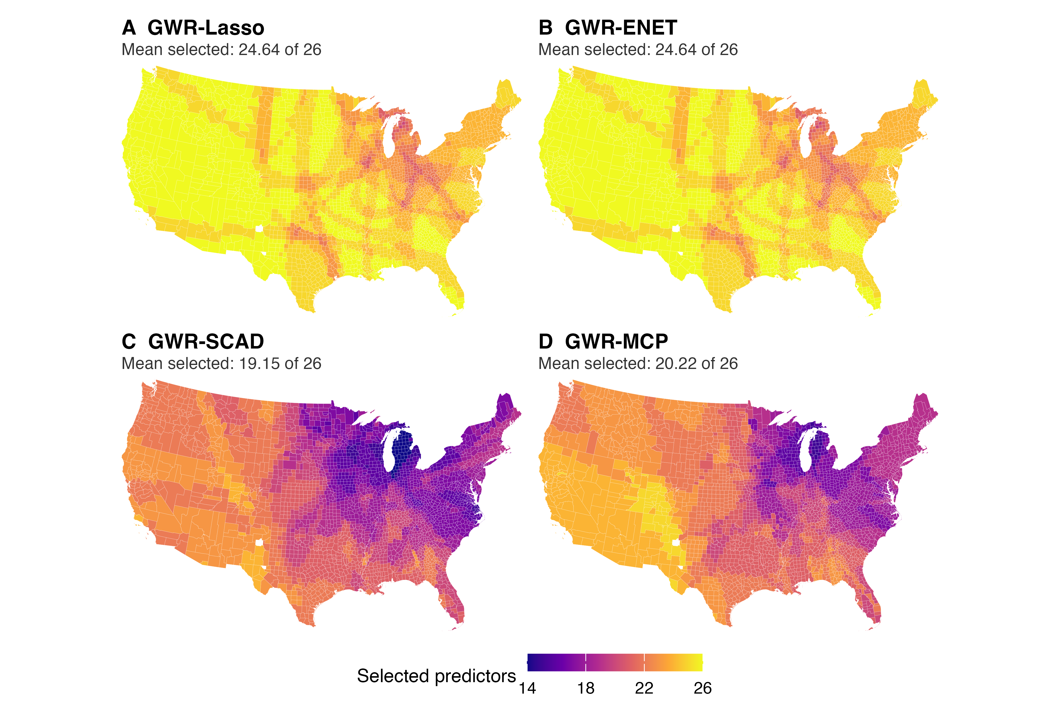
The analysis contains 26 candidate predictors. Mean local selected counts are 24.64 for GWR-Lasso, 24.64 for GWR-ENET, 19.15 for GWR-SCAD and 20.22 for GWR-MCP. These are descriptive results for this application; lower counts alone do not establish better variable recovery or prediction. Ridge is absent from this selection figure because it does not induce exact coefficient sparsity.

This image is the checked manuscript’s Figure 1, copied without modification. It is a result of the completed empirical study, rather than the small software demonstration. pkgdown/figure-provenance.json records its source filename and checksum.

Reproduce and interpret

The paper reproduction guide links to the full application, its inputs, historical package engine, checkpoint validation and publication renderer. After a complete validated application run, the documented real-data report command produces the study report from those results. Consult the manuscript and supplement for the selection convention, tuning procedure and empirical interpretation.

The getting-started guide demonstrates all five methods, common spatial folds, coefficient extraction and prediction at new locations with a small deterministic dataset.