Sparse Gaussian Regression with the Lambert Penalty • lambertReg

lambertReg fits sparse Gaussian regression with the Lambert penalty. A fixed penalty shape and training-only cross-validation give a direct workflow: fit a path, choose the penalty strength, inspect selected variables, and predict in the original units.

Documentation and examples

Fit a path

Explore how coefficients change as regularization varies.

Tune with CV

Choose the penalty using five-fold cross-validation and inspect its error curve.

Explain the fit

Extract selected coefficients, make predictions, and check numerical diagnostics.

Installation

R (>= 4.1.0), Rcpp, and an R-compatible C++ compiler are required. Clone the public repository and install the package:

git clone https://github.com/byuzbasi/lambertReg.git
R CMD INSTALL lambertReg

To include the worked vignette, make knitr, rmarkdown, and Pandoc available, then build before installing:

R CMD build lambertReg
R CMD INSTALL lambertReg_0.1.10.tar.gz

A small example

library(lambertReg)
set.seed(42)
x <- matrix(rnorm(100 * 8), 100, 8)
colnames(x) <- paste0("x", 1:8)
y <- 2 * x[, 1] - x[, 2] + 0.5 * x[, 3] + rnorm(100)
train <- 1:80
foldid <- sample(rep(1:5, length.out = length(train)))

fit <- cv.lambert(x[train, ], y[train], foldid = foldid)
coef(fit)
predict(fit, newx = x[-train, ])
plot(fit)

The 20 held-out observations do not enter scaling or tuning. The default CV path contains 60 penalty fractions. Predictors are centered and scaled within each training fold; coefficients and predictions are returned on the original scale. fit$lambda.min is the selected penalty for the full training sample.

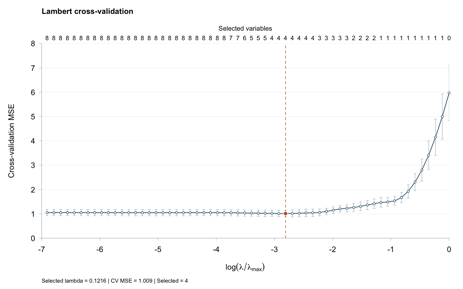
CV error for the seed-42 synthetic example, with fold-based error bars and selected-variable counts.

This is a reproducible synthetic demonstration, not an empirical result from the paper. Error bars show one descriptive fold-based standard error. The orange marker identifies the CV-selected penalty.

Paths, predictions, and penalty tools

Task	Function
Fit a regularization path	`lambert()`
Select the penalty strength	`cv.lambert()`
Extract coefficients or predict	`coef()`, `predict()`
Plot CV error or coefficient paths	`plot()`
Evaluate the penalty or scalar update	`lambert_penalty()`, `lambert_threshold()`

plot(fit, style = "paper")
plot(fit, type = "coefficients", labels = TRUE)

The shape is fixed at c = 1; CV chooses the penalty strength. Plotting uses stored results. The nonconvex solver seeks a stationary solution; inspect fit$ok, fit$partial_search, and fit$cv_diagnostics before interpreting a fit.

Guides and reproducibility

Getting started: fitting, tuning, prediction, and diagnostics.
Example gallery: CV and coefficient-path plots.
Data and reproduction guide: input definitions, saved folds, and reproducible outputs.
Runnable example: the seed-42 demonstration, including input data, plots, and a SHA-256 manifest.
Validation scope and contribution guide.

vignette("introduction", package = "lambertReg")
?cv.lambert
citation("lambertReg")

Citation and support

Use citation("lambertReg") or the repository’s CITATION.cff. The associated paper is The Lambert Penalty: Logarithmic Shrinkage for Sparse Regression (Bahadir Yuzbasi, 2026), arXiv preprint arXiv:2610.09627 [stat.ME].

Source code · Report an issue · Version notes

GPL-3. Maintainer: Bahadir Yuzbasi b.yzb@hotmail.com.